K-Nearest Neighbors (KNN) Algorithm

The Nearest Neighbors algorithm is among the simplest supervised machine learning algorithms studied in data science. Widely used for classification and regression tasks, we will talk about two types of Nearest Neighbors algorithms: 1-Nearest Neighbor and K-Nearest Neighbors (KNN). K-NN is just an extension of 1-NN, where instead of looking at the single nearest neighbor, we look at the K nearest neighbors to make a prediction.

1. Key Concepts¶

While KNN algorithm is a universal function approximator under certain conditions, it is not a parametric model. It does not learn a function from the training data; instead, it memorizes or stores the training data (inputs and labels).

$D = \{(x_i, y_i)\}_{i=1}^N$

Where $x_i$ is the input and $y_i$ is the corresponding label. And $N$ is the number of training samples.

The K-NN is called a lazy learner because it does not learn a model during the training phase. Instead, it simply stores the training data and waits until it receives a query (a new input) to make a prediction. When a new input is given, K-NN looks at the K nearest neighbors in the training data and makes a prediction based on the majority class (for classification) or the average of the neighbors’ values (for regression). The exact mechanics will be explained in the section.

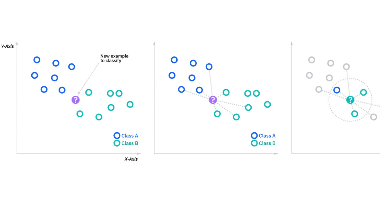
Figure 1: Illustration of the algorithm in two-dimensional space.

Source : What is the k-nearest neighbors algorithm?, IBM, https://www.ibm.com/think/topics/knn#684929711

The mathematical formulation of the K-NN algorithm can be expressed as follows:

$f(x) = \frac{1}{K} \sum_{i=1}^{K} y_i$

Where:

$f(x)$ is the predicted output for the input $x$ .
$K$ is the number of nearest neighbors considered.
$y_i$ is the label of the $i$ -th nearest neighbor.

In classification tasks, the output will be a class label determined by the majority vote among the K nearest neighbors. In regression tasks, the output will be a continuous value calculated as the average of the K nearest neighbors’ values.

But how do we determine the nearest neighbors?

2. Distance Metrics¶

In order to determine the nearest neighbors, we need to define a distance metric that quantifies the similarity between data points. These distance metrics help to find decisions boundaries in the feature space.

Some common distance metrics used in KNN include:

Euclidean Distance: Most commonly used, it is the straight-line distance between two points in a multi-dimensional space. It is calculated as:

$d(x, y) = \sqrt{\sum_{i=1}^{n} (x_i - y_i)^2}$

Where $x$ and $y$ are two data points, and $n$ is the number of features.

Manhattan Distance: Also known as the L1 distance, it is the sum of the absolute differences between the coordinates of two points. It is calculated as:

$d(x, y) = \sum_{i=1}^{n} |x_i - y_i|$

Minkowski Distance: A generalization of both Euclidean and Manhattan distances, it is calculated as:

$d(x, y) = \left( \sum_{i=1}^{n} |x_i - y_i|^p \right)^{1/p}$

Hamming Distance: Used for categorical data, it counts the number of positions at which the corresponding elements are different. It is calculated as:

$d(x, y) = \sum_{i=1}^{n} \delta(x_i, y_i)$

Where $\delta(x_i, y_i)$ is 1 if $x_i \neq y_i$ and 0 otherwise.

Note : The choice of the distance metric to use depends on the nature of the data and the specific problem at hand. For example, Euclidean distance is suitable for continuous numerical data, while Hamming distance is more appropriate for categorical data. It is important to experiment with different distance metrics to find the one that works best for your specific dataset and task.

The value of k is a crucial hyperparameter in the KNN algorithm. It determines how many nearest neighbors are considered when making a prediction. The choice of k can significantly impact the performance of the model.

For example, if k=1, the algorithm will simply predict the label of the nearest neighbor, which can lead to overfitting if the training data is noisy. On the other hand, if k is too large, the algorithm may include too many neighbors that are not relevant to the prediction, leading to underfitting.

Defining the optimal value of k is often done through experimentation and cross-validation. A common approach is to try different values of k and evaluate the model’s performance using a validation set or through cross-validation techniques. The value of k that yields the best performance on the validation set is typically chosen as the optimal k for the model. Overall, it is recommended to have an odd value for k to avoid ties in classification tasks, and to choose a value that balances the bias-variance trade-off for the specific dataset and problem at hand.

3. Pseudo-algorithm¶

$\mathcal{D} \leftarrow$ training set of $n$ labeled instances $(\mathbf{x}_i, y_i)$
$\mathbf{x} \leftarrow$ new unlabeled instance to classify
$k \leftarrow$ number of nearest neighbors to consider ( $\ge 1$ )
$\text{dist}(\mathbf{x}, \mathbf{x}_i) \leftarrow$ distance function to measure similarity between instances
function $\text{KNN\_Classify}(\mathbf{x}, \mathcal{D}, k)$
for each $(\mathbf{x}_i, y_i) \in \mathcal{D}$ do
$\quad d_i \leftarrow \text{dist}(\mathbf{x}, \mathbf{x}_i)$
end for
$\mathcal{I} \leftarrow$ indices of the $k$ smallest values in $\{d_1, \dots, d_n\}$
$\hat{y} \leftarrow \text{mode}(\{y_i : i \in \mathcal{I}\})$
return $\hat{y}$
end

4. Implementation¶

For this implementation, we will use the Iris dataset, which is a commonly used dataset in machine learning. It consists of 150 samples of iris flowers, with 4 features (sepal length, sepal width, petal length, petal width) and 3 classes (setosa, versicolor, virginica).

import pandas as pd
from sklearn.datasets import load_iris
from ifri_mini_ml_lib.preprocessing.preparation import DataSplitter

iris = load_iris()
X = pd.DataFrame(iris.data, columns=iris.feature_names)
y = pd.Series(iris.target)

X.head()

# Split the data into training and testing sets
splitter = DataSplitter(seed=42)
X_train, X_test, y_train, y_test = splitter.train_test_split(X, y, test_size=0.2)

With Scikit-learn¶

# time to mesure the execution time
import time

from sklearn.neighbors import KNeighborsClassifier

start_1 = time.perf_counter()
clf = KNeighborsClassifier(n_neighbors=3)
clf.fit(X_train, y_train)
end_1 = time.perf_counter()

With ifri-mini-ml-lib¶

from ifri_mini_ml_lib.classification import KNN

start_2 = time.perf_counter()
knn = KNN(k=3)
knn.fit(X_train, y_train)
end_2 = time.perf_counter()

# Predict the labels for the test set
y_pred_1 = clf.predict(X_test)
y_pred_2 = knn.predict(X_test)

# Evaluate the accuracy of the model
from ifri_mini_ml_lib.metrics.classification import accuracy, f1_score, recall, precision

# Compare the predictions with the true labels
accuracy_1 = accuracy(y_test, y_pred_1)
accuracy_2 = accuracy(y_test, y_pred_2)

f1_score_1 = f1_score(y_test, y_pred_1)
f1_score_2 = f1_score(y_test, y_pred_2)

recall_1 = recall(y_test, y_pred_1)
recall_2 = recall(y_test, y_pred_2)

precision_1 = precision(y_test, y_pred_1)
precision_2 = precision(y_test, y_pred_2)

# Table of results
results = pd.DataFrame({
    'Metric': ['Accuracy', 'F1 Score', 'Recall', 'Precision', 'Time'],
    'Scikit-learn': [accuracy_1, f1_score_1, recall_1, precision_1, (end_1 - start_1)],
    'ifri-mini-ml-lib': [accuracy_2, f1_score_2, recall_2, precision_2, (end_2 - start_2)],
})

results.T

5. Interactive demo¶

from ipywidgets import interact, IntSlider, Dropdown
from notebooks.classification.utils import plot_knn

interact(
    plot_knn,
    k=IntSlider(min=1, max=15, step=1, value=3, description='k Value:'),
    metric=Dropdown(
        options=['euclidean', 'manhattan', 'chebyshev', 'minkowski'],
        value='euclidean',
        description='Distance:'
    ),
    library=Dropdown(
        options=['sklearn', 'ifri_mini_ml_lib'],
        value='sklearn',
        description='Library:'
    )
);

Above is an interactive demo that allows you to visualize the decision boundaries of the KNN algorithm with different values of k and distance metrics. You can also choose between the implementation from Scikit-learn and ifri-mini-ml-lib to see how they compare in terms of decision boundaries.

6. Real-life applications¶

Because of its simplicity and capability to handle both classification and regression tasks, KNN is widely used in various domains.

Healthcare and Medical Diagnosis: KNN can be used to classify medical conditions based on patient data, such as symptoms, test results, and medical history. For example, it can help in diagnosing diseases by comparing a patient’s data with that of known cases. (ex: https://www.nature.com/articles/s41598-022-10358-x)
Recommender Engines: In marketplace and streaming platorms (like Amazon, Netflix), KNN can be used to recommend products or content to users based on their preferences and the preferences of similar users.
Computer Vision and Pattern Recognition : Researchers have developped highly accurate KNN-based models for image classification, object recognition, and facial recognition tasks. KNN can be used to classify images based on their features and similarities to other images in the training dataset.
Finance and Fraud Detection: KNN can be used to detect fraudulent transactions by comparing new transactions with historical data. It can identify patterns and anomalies that may indicate fraudulent activity.

This list is not exhaustive, and KNN can be applied to many other domains and tasks where classification or regression is needed. Its simplicity and effectiveness make it a popular choice for various applications in machine learning.

7. Limitations and Challenges¶

While KNN is a powerful algorithm, it has some limitations and challenges that should be considered when applying it to real-world problems.

Curse of Dimensionality: As the number of features increases, the distance between data points becomes less meaningful, and the algorithm’s performance can degrade. This is because in high-dimensional spaces, all points tend to be equidistant from each other, making it difficult for KNN to find meaningful neighbors.
Computational Complexity: KNN can be computationally expensive, especially for large datasets, as it requires calculating the distance between the query point and all points in the training dataset. This can lead to slow predictions, particularly when the dataset is large.
Sensitivity to Noise: KNN can be sensitive to noisy data and outliers, as they can significantly affect the distance calculations and lead to incorrect predictions. If the training data contains a lot of noise, KNN may struggle to find the correct neighbors and make accurate predictions. Techniques such as data preprocessing, feature selection, and outlier detection can help mitigate this issue.

Overall, while KNN is a simple and effective algorithm, it is important to be aware of its limitations and challenges when applying it to real-world problems. It may not always be the best choice for every task, and it is important to consider the specific characteristics of the dataset and the problem at hand when choosing an appropriate algorithm.

8. References¶

What is the k-nearest neighbors algorithm?, IBM, https://www.ibm.com/think/topics/knn#684929711
KNN Lectures Notes, Sebastian Raschka, https://sebastianraschka.com/pdf/lecture-notes/stat479fs18/02_knn_notes.pdf
Examples applications of KNN, Towards Data Science, https://towardsdatascience.com/example-applications-of-k-nearest-neighbors-e6e47cd73f1f/
Neighbors, Scikit-learn, https://scikit-learn.org/stable/modules/neighbors.html